Tutorial 4: The use and estimation of covariance
As seen in Tutorial 3, DISSTANS can also make use of data variance and covariance if provided in the timeseries. While this was not specifically addressed in the previous tutorial, taking advantage of that information can improve the fit to the data and provide insight into fitted model parameter covariances, especially when there is a large amount of correlation across components. This tutorial will explore this with a small synthetic network that has large but strongly correlated errors.
Making a noisy network
The setup should be familiar:
>>> # initialize RNG
>>> import numpy as np
>>> rng = np.random.default_rng(0)
>>> # create network in shape of a circle
>>> from disstans import Network, Station
>>> net_name = "CircleVolcano"
>>> num_stations = 8
>>> station_names = [f"S{i:1d}" for i in range(1, num_stations + 1)]
>>> angles = np.linspace(0, 2*np.pi, num=num_stations, endpoint=False)
>>> lons, lats = np.cos(angles)/10, np.sin(angles)/10
>>> net = Network(name=net_name)
>>> for (istat, stat_name), lon, lat in zip(enumerate(station_names), lons, lats):
...     net[stat_name] = Station(name=stat_name, location=[lat, lon, 0.0])
>>> # create timevector
>>> import pandas as pd
>>> t_start_str = "2000-01-01"
>>> t_end_str = "2001-01-01"
>>> timevector = pd.date_range(start=t_start_str, end=t_end_str, freq="1D")
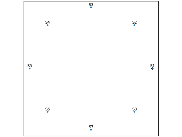
This will create a network of 8 stations, arranged in a circle, and define the timespan we’re interested in.
In the next step, like in the previous tutorial, we will create a function that returns model parameters for the generation of the synthetic data. The function most crucially though will also create the correlated noise. It does that by defining a (constant) noise covariance matrix, and then rotating that based on the location of the station. The result will be a noise covariance ellipse that will also have its long side pointed outwards of the center of the network. The function will both return the noise realization for a station, as well as the data variance and covariance vectors.
For the signal itself, we will have a constant secular motion across the network, and in the first half of the timespan, a transient outwards of the center.
The function will look like this:
>>> def generate_model_and_noise(angle, rng):
...     # get dimensions
...     n1 = int(np.floor(timevector.size / 2))
...     n2 = int(np.ceil(timevector.size / 2))
...     # rotation matrix
...     R = np.array([[np.cos(angle), -np.sin(angle)], [np.sin(angle), np.cos(angle)]])
...     # secular motion
...     p_sec = np.array([[0, 0], [6, 0]])
...     # transient motion, only in first half
...     p_vol = np.array([[8, 0]])
...     p_vol_rot = p_vol @ R.T
...     # correlated error in direction of angle in first half
...     cov_cor = np.diag([10, 3])
...     cov_rot = R @ cov_cor @ R.T
...     noise_cor = np.empty((timevector.size, 2))
...     noise_cor[:n1, :] = rng.multivariate_normal(mean=(0, 0), cov=cov_rot, size=n1)
...     # not correlated in second half
...     cov_uncor = np.diag([3, 3])
...     noise_cor[-n2:, :] = rng.multivariate_normal(mean=(0, 0), cov=cov_uncor, size=n2)
...     # make uncertainty columns
...     var_en = np.empty((timevector.size, 2))
...     cov_en = np.empty((timevector.size, 1))
...     var_en[:n1, :] = np.diag(cov_rot).reshape(1, 2) * np.ones((n1, 2))
...     var_en[-n2:, :] = np.diag(cov_uncor).reshape(1, 2) * np.ones((n2, 2))
...     cov_en[:n1, :] = cov_rot[0, 1] * np.ones((n1, 1))
...     cov_en[-n2:, :] = cov_uncor[0, 1] * np.ones((n2, 1))
...     return p_sec, p_vol_rot, noise_cor, var_en, cov_en
Now we can create the “true” timeseries, as well as a “data” timeseries that contains
noise. As before, we first create the Model objects, then evaluate
them to get the two timeseries, then make Timeseries objects
out of them, add them to the station as the two timeseries 'Truth' and
'Displacement', and finally add the model objects to the station as well.
>>> from copy import deepcopy
>>> from disstans import Timeseries
>>> from disstans.models import Arctangent, Polynomial, SplineSet
>>> mdl_coll, mdl_coll_synth = {}, {}  # containers for the model objects
>>> synth_coll = {}  # dictionary of synthetic data & noise for each stations
>>> for station, angle in zip(net, angles):
...     # think of some model parameters
...     gen_data = {}
...     p_sec, p_vol, gen_data["noise"], var_en, cov_en = \
...         generate_model_and_noise(angle, rng)
...     # create model objects
...     mdl_sec = Polynomial(order=1, time_unit="Y", t_reference=t_start_str)
...     # Arctangent is for the truth, SplineSet are for how we will estimate them
...     mdl_vol = Arctangent(tau=20, t_reference="2000-03-01")
...     mdl_trans = SplineSet(degree=2,
...                           t_center_start=t_start_str,
...                           t_center_end=t_end_str,
...                           list_num_knots=[7, 13])
...     # collect the models in the dictionary
...     mdl_coll_synth[station.name] = {"Secular": mdl_sec}
...     mdl_coll[station.name] = deepcopy(mdl_coll_synth[station.name])
...     mdl_coll_synth[station.name].update({"Volcano": mdl_vol})
...     mdl_coll[station.name].update({"Transient": mdl_trans})
...     # only the model objects that will not be associated with the station
...     # get their model parameters input
...     mdl_sec.read_parameters(p_sec)
...     mdl_vol.read_parameters(p_vol)
...     # now, evaluate the models...
...     gen_data["truth"] = (mdl_sec.evaluate(timevector)["fit"] +
...                          mdl_vol.evaluate(timevector)["fit"])
...     gen_data["data"] = gen_data["truth"] + gen_data["noise"]
...     synth_coll[station.name] = gen_data
...     # ... and assign them to the station as timeseries objects
...     station["Truth"] = \
...         Timeseries.from_array(timevector=timevector,
...                               data=gen_data["truth"],
...                               src="synthetic",
...                               data_unit="mm",
...                               data_cols=["E", "N"])
...     station["Displacement"] = \
...         Timeseries.from_array(timevector=timevector,
...                               data=gen_data["data"],
...                               var=var_en,
...                               cov=cov_en,
...                               src="synthetic",
...                               data_unit="mm",
...                               data_cols=["E", "N"])
...     # finally, we give the station the models to fit
...     station.add_local_model_dict(ts_description="Displacement",
...                                  model_dict=mdl_coll[station.name])
Let’s have a quick look at the network and its timeseries by using:
>>> net.gui()
Which will yield the following map:
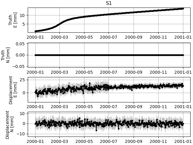
And for station S1, we see the following two timeseries:
Fitting the models with the spatial L0 solver
The following steps are nothing new - we will solve for model parameters with the
spatialfit() method. However, this time we’re explicitly
specifying if we want the solver to use data (co)variance.
This first run doesn’t use either the data variance or covariance, and we will save the estimated linear velocity parameter and covariance for every station and component for later comparison.
>>> # define a reweighting function
>>> from disstans.solvers import LogarithmicReweighting
>>> rw_func = LogarithmicReweighting(1e-8, scale=10)
>>> # solve without using the data variance
>>> stats = net.spatialfit("Displacement",
...                        penalty=10,
...                        spatial_l0_models=["Transient"],
...                        spatial_reweight_iters=20,
...                        reweight_func=rw_func,
...                        use_data_variance=False,
...                        use_data_covariance=False,
...                        formal_covariance=True,
...                        verbose=True)
Calculating scale lengths
...
Done
>>> net.evaluate("Displacement", output_description="Fit_onlydata")
>>> # save estimated velocity components
>>> vel_en_est = {}
>>> vel_en_est["onlydata"] = \
...     np.stack([s.models["Displacement"]["Secular"].parameters[1, :] for s in net])
>>> # save estimated velocity covariances
>>> cov_en_est = {}
>>> cov_en_est["onlydata"] = \
...     np.stack([s.models["Displacement"]["Secular"].cov[[2, 3, 2], [2, 3, 3]] for s in net])
In the next two runs, we will first add the variance, and then the covariance. At the end, for future comparison, we save the estimated parameters and covariances.
>>> # solve using the data variance
>>> stats = net.spatialfit("Displacement",
...                        penalty=10,
...                        spatial_l0_models=["Transient"],
...                        spatial_reweight_iters=20,
...                        reweight_func=rw_func,
...                        use_data_variance=True,
...                        use_data_covariance=False,
...                        formal_covariance=True,
...                        verbose=True)
Calculating scale lengths
...
Done
>>> net.evaluate("Displacement", output_description="Fit_withvar")
>>> # save estimated velocity components
>>> vel_en_est["withvar"] = \
...     np.stack([s.models["Displacement"]["Secular"].parameters[1, :] for s in net])
>>> # save estimated velocity covariances
>>> cov_en_est["withvar"] = \
...     np.stack([s.models["Displacement"]["Secular"].cov[[2, 3, 2], [2, 3, 3]] for s in net])
>>> # solve with the data variance and covariance
>>> stats = net.spatialfit("Displacement",
...                        penalty=10,
...                        spatial_l0_models=["Transient"],
...                        spatial_reweight_iters=20,
...                        reweight_func=rw_func,
...                        use_data_variance=True,
...                        use_data_covariance=True,
...                        formal_covariance=True,
...                        verbose=True)
Calculating scale lengths
...
Done
>>> net.evaluate("Displacement", output_description="Fit_withvarcov")
>>> # save estimated velocity components
>>> vel_en_est["withvarcov"] = \
...     np.stack([s.models["Displacement"]["Secular"].parameters[1, :] for s in net])
>>> # save estimated velocity covariances
>>> cov_en_est["withvarcov"] = \
...     np.stack([s.models["Displacement"]["Secular"].cov[[2, 3, 2], [2, 3, 3]] for s in net])
Notice that right off the bat, including the variance and covariance data in the estimation has reduced the number of iterations necessary, and has pushed the spatial solver to select only a single spline per component and station to model the transient.
Just to get an idea of the fit, we can again use the GUI function to show us the fits and scalograms:
>>> net.gui(station="S2", timeseries=["Displacement"],
...     scalogram_kw_args={"ts": "Displacement", "model": "Transient", "cmaprange": 3})
For station S2, we get the following model fit and scalogram:


Quality of the fits
We now want to see how close we got to the true secular velocity. For that, we first need to collect the true velocity vectors at all stations:
>>> vel_en_true = np.stack([mdl_coll_synth[s]["Secular"].parameters[1, :]
...                         for s in station_names])
>>> norm_true = np.sqrt(np.sum(vel_en_true**2, axis=1))
Now we can calculate the deviation of the estimate both in terms of magnitude and direction from the true values, and print the estimated model parameter covariance:
>>> err_stats = {}
>>> for title, case in \
...     zip(["Data", "Data + Variance", "Data + Variance + Covariance"],
...         ["onlydata", "withvar", "withvarcov"]):
...     # error statistics
...     print(f"\nError Statistics for {title}:")
...     # get amplitude errors
...     norm_est = np.sqrt(np.sum(vel_en_est[case]**2, axis=1))
...     err_amp = norm_est - norm_true
...     # get absolute angle error by calculating the angle between the two vectors
...     dotprodnorm = (np.sum(vel_en_est[case] * vel_en_true, axis=1) /
...                    (norm_est * norm_true))
...     err_angle = np.rad2deg(np.arccos(dotprodnorm))
...     # make error dataframe and print
...     err_df = pd.DataFrame(index=station_names,
...                           data={"Amplitude": err_amp, "Angle": err_angle})
...     print(err_df)
...     # print rms of both
...     print(f"RMS Amplitude: {np.sqrt(np.mean(err_amp**2)):.11g}")
...     print(f"RMS Angle: {np.sqrt(np.mean(err_angle**2)):.11g}")
...     # print covariances
...     print("Secular (Co)Variances")
...     print(pd.DataFrame(index=station_names,
...                        data=cov_en_est[case],
...                        columns=["E-E", "N-N", "E-N"]))

Error Statistics for Data:
    Amplitude      Angle
S1   2.598428   1.215275
S2   0.505623   4.063633
S3  -0.823852  11.933309
S4  -1.309459  14.540778
S5  -1.895504  10.011640
S6   0.477857   8.026414
S7   0.292104  12.141594
S8   0.863249   6.090901
RMS Amplitude: 1.3253632716
RMS Angle: 9.4934302719
Secular (Co)Variances
         E-E       N-N  E-N
S1  0.063691  0.063691  0.0
S2  0.063691  0.063691  0.0
S3  0.063691  0.063691  0.0
S4  0.063691  0.063691  0.0
S5  0.088382  0.063691  0.0
S6  0.063691  0.063691  0.0
S7  0.063691  0.063691  0.0
S8  0.063691  0.063691  0.0

Error Statistics for Data + Variance:
    Amplitude     Angle
S1   1.680626  1.263873
S2   0.245351  1.477345
S3  -0.928216  2.238697
S4  -0.985113  6.066963
S5  -1.082151  7.696245
S6   0.995734  3.697095
S7   0.106339  1.188509
S8   0.572923  3.609512
RMS Amplitude: 0.94992227405
RMS Angle: 4.0764805213
Secular (Co)Variances
         E-E       N-N  E-N
S1  0.397303  0.226716  0.0
S2  0.327963  0.327963  0.0
S3  0.226716  0.397303  0.0
S4  0.327963  0.327963  0.0
S5  0.397303  0.226716  0.0
S6  0.327963  0.327963  0.0
S7  0.226716  0.397303  0.0
S8  0.327963  0.327963  0.0

Error Statistics for Data + Variance + Covariance:
    Amplitude      Angle
S1   1.888550   1.969501
S2   0.414432   2.517659
S3  -0.811653   4.516261
S4  -0.993368  10.887050
S5  -1.305148   6.773861
S6   0.738884   5.765371
S7   0.169693   3.082705
S8   0.815215   5.680584
RMS Amplitude: 1.0202124819
RMS Angle: 5.8098923752
Secular (Co)Variances
         E-E       N-N           E-N
S1  0.397303  0.226716 -1.915294e-16
S2  0.312009  0.312009  8.529381e-02
S3  0.226716  0.397303 -1.291082e-15
S4  0.312009  0.312009 -8.529381e-02
S5  0.397303  0.226716  9.883866e-17
S6  0.312009  0.312009  8.529381e-02
S7  0.097160  0.397303  3.061551e-16
S8  0.312009  0.312009 -8.529381e-02
Including the (co)variance has decreased our misfit slightly. However, including the variance information in the fitting process has led to smaller formal uncertainties in the fitted model parameters. Finally, comparing the covariance case with the variance case, we have furthermore gained insight that the East-North components of the velocity for stations S2, S4, S6, and S8 are strongly correlated.
Correlation of parameters
Let’s have a closer look at how we can estimate the error in our prediction (i.e. fitted
timeseries). By default, if the formal covariance is estimated by the solver, that formal
uncertainty is passed on to the ModelCollection object where
we can look at it in the cov property.
We can save it for later like this:
>>> spat_cov = {sta_name: net[sta_name].models["Displacement"].cov
...             for sta_name in station_names}
Whenever then the model gets evaluated, it will also map that model parameter uncertainty into the data space (the blue shaded region in the figure above). For the case where the dictionary of splines is overcomplete, there will undoubtedly be a large correlation between splines - this is the entire reason we need L1/L0 regularization to deal with the degeneracy.
Let’s have a look at the correlation matrix, by first defining a simple plotting function:
>>> import matplotlib.pyplot as plt
>>> from cmcrameri import cm as scm
>>> from disstans.tools import cov2corr
>>> # define a plotting function for repeatability
>>> def corr_plot(cov, title, fname_corr):
...     plt.imshow(cov2corr(cov), cmap=scm.roma, vmin=-1, vmax=1)
...     plt.colorbar(label="Correlation Coefficient $[-]$")
...     plt.title("Correlation: " + title)
...     plt.xlabel("Parameter index")
...     plt.ylabel("Parameter index")
...     plt.savefig(fname_corr)
...     plt.close()
(We don’t want to use plot_covariance() here since
later we will have an empirical covariance that we have to plot ourselves anyways.)
And now running it:
>>> corr_plot(spat_cov["S2"], "Spatial L0 at S2", "tutorial_4d_corr_S2.png")
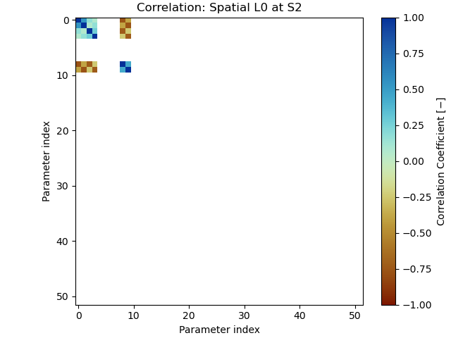
As one can see, there is a strong tradeoff between the linear terms (indices 2-3) and the splines in the rest of the dictionary. Note that all but one splines have zero-valued parameters, so the uncertainty is not directly visible in the timeseries.
Note
The empty columns and rows in the correlation matrix are a result of how the
model parameter covariance matrix is estimated by
lasso_regression(). Because the computation requires a
matrix inverse, but the problem is not full rank (because the splines are an
overcomplete dictionary), some entries have to be set to zero before the inversion,
yielding in empty correlation rows. This threshold can be set with the
zero_threshold option.
In the following sections, let’s explore other ways we can get a sense of our parameter uncertainty.
Simple linear regression with restricted spline set
The goal of the L0 solver is to find the minimum set of splines necessary to model the transient signal, based on an overcomplete dictionary of splines. Once that subset is found (e.g., the one spline in shown above), it is mathematically equivalent to just doing an unregularized, linear least squares fit.
In the correlation matrix above, we have an almost full matrix, where we see how
parameters trade off with each other, even when they have been estimated to be zero
because of our regularization. If we only wanted to see how the non-zero
parameters trade off with each other, we can “freeze” the models based on the absolute
value of their parameters. This is accomplished with the
freeze() method:
>>> net.freeze("Displacement", model_list=["Transient"], zero_threshold=1e-6)
>>> net.fitevalres("Displacement", solver="linear_regression",
...                use_data_variance=True, use_data_covariance=True,
...                formal_covariance=True)
>>> net.unfreeze("Displacement")
>>> sub_param = {sta_name: net[sta_name].models["Displacement"].par.ravel()
...              for sta_name in station_names}
>>> sub_cov = {sta_name: net[sta_name].models["Displacement"].cov
...            for sta_name in station_names}
Looking at the covariance:
>>> corr_plot(sub_cov["S2"], "Frozen local L0 at S2", "tutorial_4e_corr_S2.png")
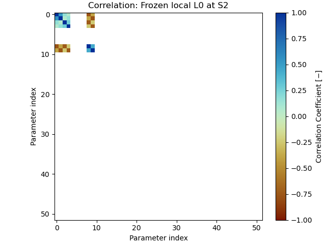
We now see how only the parameters that have been estimated have correlation entries, and again, we see the tradeoff between the one spline and the linear polynomial. The figure looks essentially the same as the previous one, confirming our mathematical approximation of the L0 regularization worked.
Empirical covariance estimation
Now that we have the formal covariance, we can also try to estimate the empirical (sample) parameters covariance. With synthetic data, this is straightforward: we create a large number of timeseries, all with the same truth signal underlying it, but with different noise realizations. We then solve for the parameters in all these cases, and use those to compute the sample covariance. If we don’t have the true original timeseries, we can still add different noise realizations at each step, but we will add the to observed timeseries (accepting that the new timeseries will have double the noise).
What we want to learn from it will then determine which of the different solvers we use. If we want to get a better understanding of the tradeoff between the actual non-zero parameters, we would repeat either the spatial L0 solution, or the unregularized solution using the restricted dictionary.
Just for demonstration purposes, however, we will do it using the local L0 solution, which will give us the understanding how different splines trade off between each other (similar to the first correlation matrix shown in this tutorial). This is because with different noise realizations, and without the spatial part of the algorithm, it is very likely that different splines will get chosen for each solution, giving us therefore a good sample set to estimate the covariance.
Now, to the code: we will first create a variable to store the estimated parameters, then start a loop, and at the end compute the sample covariance. Inside the loop, first, a new timeseries is created, then a local L0 fit is performed, and then the estimated parameters are saved.
We repeat this exercise twice, once taking advantage of our knowledge of the truth, and once purely data-based. First, truth-based:
>>> num_repeat = 100
>>> stacked_params_tru = \
...     {sta_name: np.empty((num_repeat,
...                          net[sta_name].models["Displacement"].num_parameters * 2))
...      for sta_name in station_names}
>>> # loop
>>> for i in range(num_repeat):
...     # change noise
...     for station, angle in zip(net, angles):
...         station["Displacement"].data = \
...             station["Truth"].data + generate_model_and_noise(angle, rng)[2]
...     # solve, same reweight_func, same penalty = easy
...     net.fit("Displacement", solver="lasso_regression", penalty=10,
...             reweight_max_iters=5, reweight_func=rw_func,
...             use_data_variance=True, use_data_covariance=True,
...             formal_covariance=True, progress_desc=f"Fit {i}")
...     # save
...     for sta_name in station_names:
...         stacked_params_tru[sta_name][i, :] = net[sta_name].models["Displacement"].par.ravel()
>>> # calculate empirical covariance
>>> emp_cov_tru = {sta_name: np.cov(stacked_params_tru[sta_name], rowvar=False)
...                for sta_name in station_names}
And second, data-based:
>>> num_repeat = 100
>>> stacked_params_dat = \
...     {sta_name: np.empty((num_repeat,
...                          net[sta_name].models["Displacement"].num_parameters * 2))
...      for sta_name in station_names}
>>> orig_data = {sta_name: net[sta_name]["Displacement"].data.values.copy()
...              for sta_name in station_names}
>>> # loop
>>> for i in range(num_repeat):
...     # change noise
...     for station, angle in zip(net, angles):
...         station["Displacement"].data = \
...             orig_data[station.name] + generate_model_and_noise(angle, rng)[2]
...     # solve, same reweight_func, same penalty = easy
...     net.fit("Displacement", solver="lasso_regression", penalty=10,
...             reweight_max_iters=5, reweight_func=rw_func,
...             use_data_variance=True, use_data_covariance=True,
...             formal_covariance=True, progress_desc=f"Fit {i}")
...     # save
...     for sta_name in station_names:
...         stacked_params_dat[sta_name][i, :] = net[sta_name].models["Displacement"].par.ravel()
>>> # calculate empirical covariance
>>> emp_cov_dat = {sta_name: np.cov(stacked_params_dat[sta_name], rowvar=False)
...                for sta_name in station_names}
Producing the two covariance plots:
>>> corr_plot(emp_cov_tru["S2"], "Truth-based Empirical Local L0 at S2", "tutorial_4f_corr_S2.png")
>>> corr_plot(emp_cov_dat["S2"], "Data-based Empirical Local L0 at S2", "tutorial_4g_corr_S2.png")
Let’s have a look at the two figures side-by-side:


Again, we see the strong trade-off between the splines. We also see that the data-based is relatively close to the truth-based one, which gives us at least a little bit of confidence in this approach when using real data.