Tutorial 2: Advanced Models and Fitting
This tutorial recreates the basics of the synthetic timeseries example as described in Bryan Riel’s [riel14] paper on detecting geodetic transients. To do this, we’ll be building on the workflow from the first example. This time though, we’ll first focus a bit more on making the synthetic data, before creating the station itself.
Creating more complex synthetic data
Let’s start with creating the timestamps for our synthetic data:
>>> import pandas as pd
>>> t_start_str = "2000-01-01"
>>> t_end_str = "2020-01-01"
>>> timevector = pd.date_range(start=t_start_str, end=t_end_str, freq="1D")
Next up is the model collection we’re going to use to simulate our data. This time, we’ll be using a Polynomial, Sinusoids and some Arctangents. If you have any question about this, please refer to the previous tutorial.
>>> from disstans.models import Arctangent, Polynomial, Sinusoid
>>> mdl_secular = Polynomial(order=1, t_reference=t_start_str)
>>> mdl_annual = Sinusoid(period=365.25, t_reference=t_start_str)
>>> mdl_semiannual = Sinusoid(period=365.25/2, t_reference=t_start_str)
>>> mdl_transient_1 = Arctangent(tau=100, t_reference="2002-07-01")
>>> mdl_transient_2 = Arctangent(tau=50, t_reference="2010-01-01")
>>> mdl_transient_3 = Arctangent(tau=300, t_reference="2016-01-01")
>>> mdl_coll_synth = {"Secular": mdl_secular,
...                   "Annual": mdl_annual,
...                   "Semi-Annual": mdl_semiannual,
...                   "Transient_1": mdl_transient_1,
...                   "Transient_2": mdl_transient_2,
...                   "Transient_3": mdl_transient_3}
Now, if we give these model objects to our station and perform fitting, their parameters will be overwritten (it’s one of those Python caveats). So, let’s take this time here to create a “deep” copy that we will then use for fitting. (Because fitting Arctangents is hard, we’ll omit them here, and try to approximate them with other models later.)
>>> from copy import deepcopy
>>> mdl_coll = deepcopy({"Secular": mdl_secular,
...                      "Annual": mdl_annual,
...                      "Semi-Annual": mdl_semiannual})
Now that we have a copy for safekeeping, we can add the “true” parameters to the models:
>>> import numpy as np
>>> mdl_secular.read_parameters(np.array([-20, 200/(20*365.25)]))
>>> mdl_annual.read_parameters(np.array([-5, 0]))
>>> mdl_semiannual.read_parameters(np.array([0, 5]))
>>> mdl_transient_1.read_parameters(np.array([40]))
>>> mdl_transient_2.read_parameters(np.array([-4]))
>>> mdl_transient_3.read_parameters(np.array([-20]))
We can evaluate them just like before:
>>> sum_seas_sec = mdl_secular.evaluate(timevector)["fit"] \
...                + mdl_annual.evaluate(timevector)["fit"] \
...                + mdl_semiannual.evaluate(timevector)["fit"]
>>> sum_transient = mdl_transient_1.evaluate(timevector)["fit"] \
...                 + mdl_transient_2.evaluate(timevector)["fit"] \
...                 + mdl_transient_3.evaluate(timevector)["fit"]
>>> sum_all_models = sum_seas_sec + sum_transient
Our noise this time has two components: white and colored. For the white noise,
we can just use NumPy’s default functions, but for the colored noise, we have to use
DISSTANS’s create_powerlaw_noise() function:
>>> from disstans.tools import create_powerlaw_noise
>>> rng = np.random.default_rng(0)
>>> white_noise = rng.normal(scale=2, size=(timevector.size, 1))
>>> colored_noise = create_powerlaw_noise(size=(timevector.size, 1),
...                                       exponent=1.5, seed=0) * 2
>>> sum_noise = white_noise + colored_noise
Our synthetic data is then just the sum of the ground truth sum_all_models
and the total noise sum_noise:
>>> synth_data = sum_all_models + sum_noise
Let’s have a look what we fabricated:
>>> import matplotlib.pyplot as plt
>>> from pandas.plotting import register_matplotlib_converters
>>> register_matplotlib_converters()  # improve how time data looks
>>> plt.figure()
>>> plt.plot(timevector, sum_seas_sec, c='C1', label="Seasonal + Secular")
>>> plt.plot(timevector, sum_transient, c='k', label="Transient")
>>> plt.plot(timevector, sum_noise, c='0.5', lw=0.3, label="Noise")
>>> plt.plot(timevector, synth_data, c='C0', ls='none', marker='.',
...          markersize=2, alpha=0.5, label="Synthetic Data")
>>> plt.xlabel("Time")
>>> plt.ylim(-50, 250)
>>> plt.ylabel("Displacement [mm]")
>>> plt.legend(loc="upper left")
>>> plt.savefig("tutorial_2a.png")
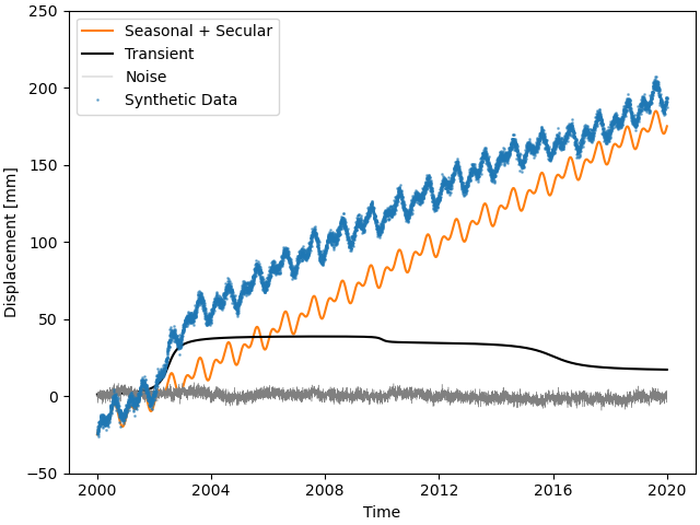
This looks close to the example in [riel14]. We can see that there are some significant transients alongside a strong secular signal, and seasonal signals plus the colored noise make it look a bit more realistic.
Spline models for transients
How do we model the transients though? For this, we will use an over-complete set
of basis functions, built by a collection of integrated B-Splines. For more on that,
see the class documentations for BSpline and
ISpline. There is a simple SplineSet
constructor class that takes care of that for us, which we’ll directly add to our
model collection from before:
>>> from disstans.models import ISpline, SplineSet
>>> mdl_coll["Transient"] = SplineSet(degree=2,
...                                   t_center_start=t_start_str,
...                                   t_center_end=t_end_str,
...                                   list_num_knots=[4, 8, 16, 32, 64, 128],
...                                   splineclass=ISpline)
It creates sets of integrated B-Splines of degree 2, with the timespan
covered to be that of our synthetic timeseries, and then divided into 4, 8, etc.
subintervals. The splineclass parameter only makes it clear that we want a set of
ISpline, but we could have omitted it, as it’s the default
behavior.
Building a Network
Now, we’re ready to build our synthetic network and add our generated data.
Again, we start by creating a Station object, but this time,
we’ll also assign it to a Network object:
>>> from disstans import Network, Station, Timeseries
>>> net_name = "TutorialLand"
>>> stat_name = "TUT"
>>> caltech_lla = (34.1375, -118.125, 263.0)
>>> net = Network(name=net_name)
>>> stat = Station(name=stat_name,
...                location=caltech_lla)
>>> net[stat_name] = stat
Note
Note that the stations internal name name does not
have to match the network’s name of that station in
stations, but it avoids confusion.
net[stat_name] = synth_stat is equivalent to
net.add_station(stat_name, synth_stat).
Add the generated timeseries (including models), as well as the ground truth to the station:
>>> ts = Timeseries.from_array(timevector=timevector,
...                            data=synth_data,
...                            src="synthetic",
...                            data_unit="mm",
...                            data_cols=["Total"])
>>> truth = Timeseries.from_array(timevector=timevector,
...                               data=sum_all_models,
...                               src="synthetic",
...                               data_unit="mm",
...                               data_cols=["Total"])
>>> stat["Displacement"] = ts
>>> stat["Truth"] = truth
>>> stat.add_local_model_dict(ts_description="Displacement",
...                           model_dict=mdl_coll)
Fitting an entire network
At this point, we’re ready to do the fitting using the simple linear non-regularized least-squares we used in the previous tutorial:
>>> net.fit(ts_description="Displacement", solver="linear_regression")
>>> net.evaluate(ts_description="Displacement", output_description="Fit_noreg")
>>> stat["Res_noreg"] = stat["Displacement"] - stat["Fit_noreg"]
>>> stat["Err_noreg"] = stat["Fit_noreg"] - stat["Truth"]
We saved a lot of lines and hassle compared to the previous fitting by using the
Network methods. We already calculated the residuals and
errors, so let’s print some statistics:
>>> _ = stat.analyze_residuals(ts_description="Res_noreg",
...                            mean=True, std=True, verbose=True)
TUT: Res_noreg                          Mean  Standard Deviation
Total-Displacement_Model_Total -2.193582e-08            2.046182
Advanced plotting
What do our fit, residuals (between the observations and our fit) and errors (between the fit and the true displacement signal) look like compared to the data and noise?
>>> from matplotlib.lines import Line2D
>>> fig, ax = plt.subplots(nrows=2, sharex=True)
>>> ax[0].plot(stat["Displacement"].data, label="Synthetic")
>>> ax[0].plot(stat["Fit_noreg"].data, label="Fit")
>>> ax[0].set_ylim(-50, 250)
>>> ax[0].set_ylabel("Displacement [mm]")
>>> ax[0].legend(loc="upper left")
>>> ax[0].set_title("No Regularization")
>>> ax[1].plot(stat["Res_noreg"].data, c='0.3', ls='none',
...         marker='.', markersize=0.5)
>>> ax[1].plot(stat["Err_noreg"].time, sum_noise, c='C1', ls='none',
...         marker='.', markersize=0.5)
>>> ax[1].plot(stat["Err_noreg"].data, c="C0")
>>> ax[1].set_ylim(-15, 15)
>>> ax[1].set_ylabel("Error [mm]")
>>> custom_lines = [Line2D([0], [0], c="0.3", marker=".", linestyle='none'),
...                 Line2D([0], [0], c="C1", marker=".", linestyle='none'),
...                 Line2D([0], [0], c="C0")]
>>> ax[1].legend(custom_lines, ["Residual", "True Noise", "Error"],
...             loc="lower left", ncol=3)
>>> fig.savefig("tutorial_2b.png")
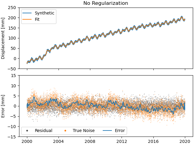
Note
As expected with any regular least-squares minimization, the residuals look like a zero-mean Gaussian distribution. The true noise, plotted for comparison, contains colored noise, and therefore is not Gaussian. Because our solver has no way of knowing what is true noise and small transient signals, it assumes that all the transient it sees are part of the displacement signal to fit. Therefore, our error tracks the noise. This behaviour will not change significantly throughout this second tutorial, but will be addressed in the third tutorial.
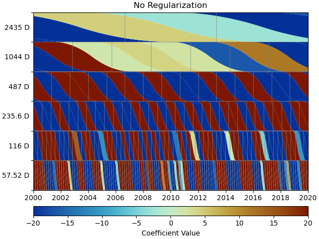
We can use a scalogram (see make_scalogram()) to visualize
the coefficient values of our spline collection, and quickly understand that without
regularization, the set is quite heavily populated in order to minimize the residuals:
>>> fig, ax = stat.models["Displacement"]["Transient"].make_scalogram(t_left=t_start_str,
...                                                                   t_right=t_end_str,
...                                                                   cmaprange=20)
>>> ax[0].set_title("No Regularization")
>>> fig.savefig("tutorial_2c.png")
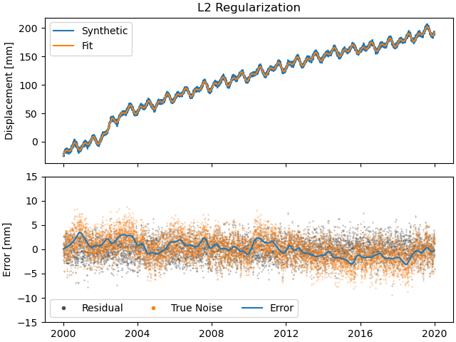
Repeat with L2 regularization
Now, we can do the exact same thing as above, but choose a ridge regression (L2-regularized) solver:
>>> net.fit(ts_description="Displacement", solver="ridge_regression", penalty=10)
>>> net.evaluate(ts_description="Displacement", output_description="Fit_L2")
>>> stat["Res_L2"] = stat["Displacement"] - stat["Fit_L2"]
>>> stat["Err_L2"] = stat["Fit_L2"] - stat["Truth"]
Giving us the statistics:
>>> _ = stat.analyze_residuals(ts_description="Res_L2",
...                            mean=True, std=True, verbose=True)
TUT: Res_L2                             Mean  Standard Deviation
Total-Displacement_Model_Total -5.627219e-09            2.088274
>>> fig, ax = plt.subplots(nrows=2, sharex=True)
>>> ax[0].plot(stat["Displacement"].data, label="Synthetic")
>>> ax[0].plot(stat["Fit_L2"].data, label="Fit")
>>> ax[0].set_ylabel("Displacement [mm]")
>>> ax[0].legend(loc="upper left")
>>> ax[0].set_title("L2 Regularization")
>>> ax[1].plot(stat["Res_L2"].data, c='0.3', ls='none',
...         marker='.', markersize=0.5)
>>> ax[1].plot(stat["Err_L2"].time, sum_noise, c='C1', ls='none',
...         marker='.', markersize=0.5)
>>> ax[1].plot(stat["Err_L2"].data, c="C0")
>>> ax[1].set_ylim(-15, 15)
>>> ax[1].set_ylabel("Error [mm]")
>>> custom_lines = [Line2D([0], [0], c="0.3", marker=".", linestyle='none'),
...                 Line2D([0], [0], c="C1", marker=".", linestyle='none'),
...                 Line2D([0], [0], c="C0")]
>>> ax[1].legend(custom_lines, ["Residual", "True Noise", "Error"],
...             loc="lower left", ncol=3)
>>> fig.savefig("tutorial_2d.png")
>>> fig, ax = stat.models["Displacement"]["Transient"].make_scalogram(t_left=t_start_str,
...                                                                   t_right=t_end_str,
...                                                                   cmaprange=20)
>>> ax[0].set_title("L2 Regularization")
>>> fig.savefig("tutorial_2e.png")
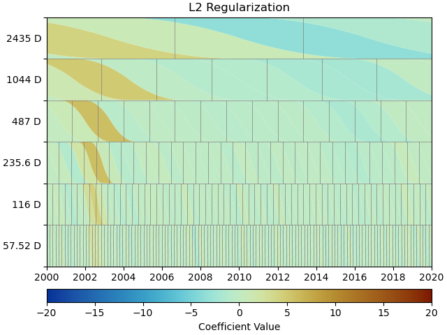
We can see that L2 regularization has significantly reduced the magnitude of the splines used in the fitting, and the fit overall (see the residual statistics) appears to be better. However, most splines are actually non-zero. This might produced the best fit, but our physical knowledge of the processes happening tell us that our station is not always moving - there are discrete processes. A higher penalty parameter might make those parameters even smaller, but they will not become significantly sparser.
Let’s save the parameter values of the transient spline model such that we can compare them later to cases with different regularizations:
>>> params_transient_L2 = stat.models["Displacement"]["Transient"].parameters.ravel().copy()
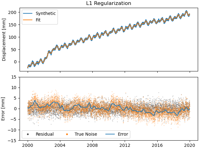
Repeat with L1 regularization
Using L1-regularized lasso regression, we finally hope to get rid of all the small, basically-zero splines in the transient dictionary:
>>> net.fit(ts_description="Displacement", solver="lasso_regression", penalty=10)
>>> net.evaluate(ts_description="Displacement", output_description="Fit_L1")
>>> stat["Res_L1"] = stat["Displacement"] - stat["Fit_L1"]
>>> stat["Err_L1"] = stat["Fit_L1"] - stat["Truth"]
Giving us the statistics:
>>> _ = stat.analyze_residuals(ts_description="Res_L1",
...                            mean=True, std=True, verbose=True)
TUT: Res_L1                             Mean  Standard Deviation
Total-Displacement_Model_Total  2.171535e-10             2.07782
>>> fig, ax = plt.subplots(nrows=2, sharex=True)
>>> ax[0].plot(stat["Displacement"].data, label="Synthetic")
>>> ax[0].plot(stat["Fit_L1"].data, label="Fit")
>>> ax[0].set_ylabel("Displacement [mm]")
>>> ax[0].legend(loc="upper left")
>>> ax[0].set_title("L1 Regularization")
>>> ax[1].plot(stat["Res_L1"].data, c='0.3', ls='none',
...         marker='.', markersize=0.5)
>>> ax[1].plot(stat["Err_L1"].time, sum_noise, c='C1', ls='none',
...         marker='.', markersize=0.5)
>>> ax[1].plot(stat["Err_L1"].data, c="C0")
>>> ax[1].set_ylim(-15, 15)
>>> ax[1].set_ylabel("Error [mm]")
>>> custom_lines = [Line2D([0], [0], c="0.3", marker=".", linestyle='none'),
...                 Line2D([0], [0], c="C1", marker=".", linestyle='none'),
...                 Line2D([0], [0], c="C0")]
>>> ax[1].legend(custom_lines, ["Residual", "True Noise", "Error"],
...             loc="lower left", ncol=3)
>>> fig.savefig("tutorial_2f.png")
>>> fig, ax = stat.models["Displacement"]["Transient"].make_scalogram(t_left=t_start_str,
...                                                                   t_right=t_end_str,
...                                                                   cmaprange=20)
>>> ax[0].set_title("L1 Regularization")
>>> fig.savefig("tutorial_2g.png")
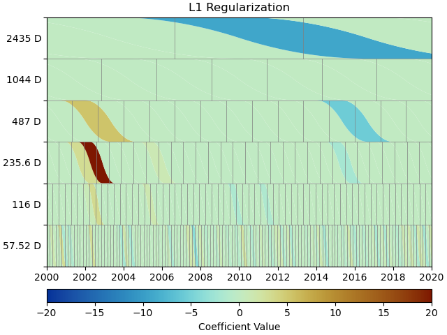
This looks much better - the scalogram now shows us that we only select splines around where we put the Arctangent models, and is close to zero otherwise. We again sae the transient model parameters for later.
>>> params_transient_L1 = stat.models["Displacement"]["Transient"].parameters.ravel().copy()
Repeat with L0 regularization
Okay, one last thing about fitting, I promise. L1 regularization aims to penalize the sum of the absolute values of our model parameters. However, that’s also not actually what we want. In fact, transient signals in the real world have no constraint to be as small as possible. However, the number of transients should be the one that is minimized. That is what is mathematically referred to as L0 regularization, but is sadly not an easy problem to solve rigorously.
However, by modifying an additional weight of each regularized parameter, that drives small
values even closer to zero, but leaves significant values unperturbed, one can approximate
such an L0 regularization by iteratively solving the L1-regularized problem. That is exactly
what the option reweight_max_iters does. You can find more information about it in
the notes of lasso_regression().
The solver requires the definition of a reweighting function - i.e., a function that
helps the solver distinguish between significant and insignificant parameters.
A reweighting function takes in parameter values, and outputs a weight to add in the
regularization process. Small parameters (insignificant) will get a very high weight
(penalty), whereas large parameters will get a weight close to zero. For more information,
refer to ReweightingFunction. Let’s define one:
>>> from disstans.solvers import InverseReweighting
>>> rw_func = InverseReweighting(1e-4, scale=1)
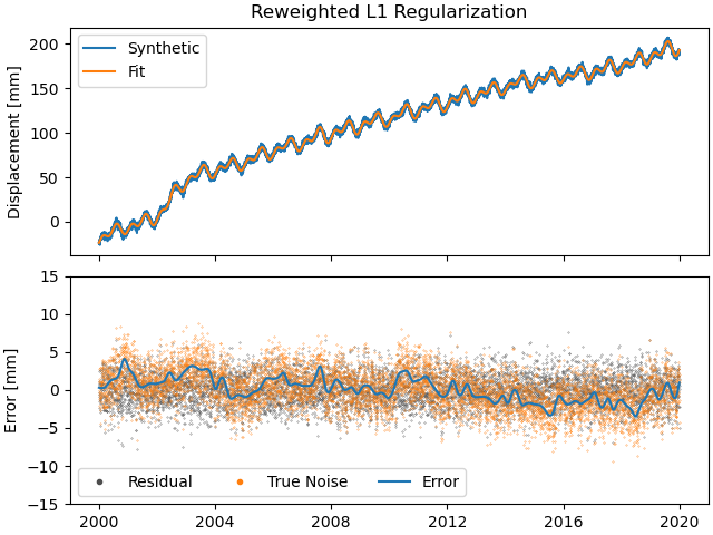
With this, we can now run the L1 solver iteratively to approximate the L0 solution:
>>> net.fit(ts_description="Displacement", solver="lasso_regression",
...         penalty=10, reweight_max_iters=20, reweight_func=rw_func)
>>> net.evaluate(ts_description="Displacement", output_description="Fit_L0")
>>> stat["Res_L0"] = stat["Displacement"] - stat["Fit_L0"]
>>> stat["Err_L0"] = stat["Fit_L0"] - stat["Truth"]
Giving us the statistics:
>>> _ = stat.analyze_residuals(ts_description="Res_L0",
...                            mean=True, std=True, verbose=True)
TUT: Res_L0                             Mean  Standard Deviation
Total-Displacement_Model_Total  4.663455e-13            2.071561
>>> fig, ax = plt.subplots(nrows=2, sharex=True)
>>> ax[0].plot(stat["Displacement"].data, label="Synthetic")
>>> ax[0].plot(stat["Fit_L0"].data, label="Fit")
>>> ax[0].set_ylabel("Displacement [mm]")
>>> ax[0].legend(loc="upper left")
>>> ax[0].set_title("Reweighted L1 Regularization")
>>> ax[1].plot(stat["Res_L0"].data, c='0.3', ls='none',
...         marker='.', markersize=0.5)
>>> ax[1].plot(stat["Err_L0"].time, sum_noise, c='C1', ls='none',
...         marker='.', markersize=0.5)
>>> ax[1].plot(stat["Err_L0"].data, c="C0")
>>> ax[1].set_ylim(-15, 15)
>>> ax[1].set_ylabel("Error [mm]")
>>> custom_lines = [Line2D([0], [0], c="0.3", marker=".", linestyle='none'),
...                 Line2D([0], [0], c="C1", marker=".", linestyle='none'),
...                 Line2D([0], [0], c="C0")]
>>> ax[1].legend(custom_lines, ["Residual", "True Noise", "Error"],
...             loc="lower left", ncol=3)
>>> fig.savefig("tutorial_2h.png")
>>> fig, ax = stat.models["Displacement"]["Transient"].make_scalogram(t_left=t_start_str,
...                                                                   t_right=t_end_str,
...                                                                   cmaprange=20)
>>> ax[0].set_title("Reweighted L1 Regularization")
>>> fig.savefig("tutorial_2i.png")
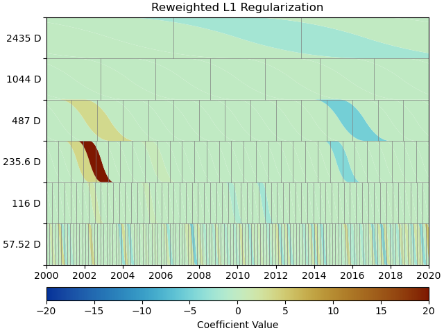
As you can see, the significant components of the splines have now been emphasized when compared to the previous scalogram, and all the values that were small but not really zero in the previous case are now really close to zero. This did not come at a significant increase in residual variance.
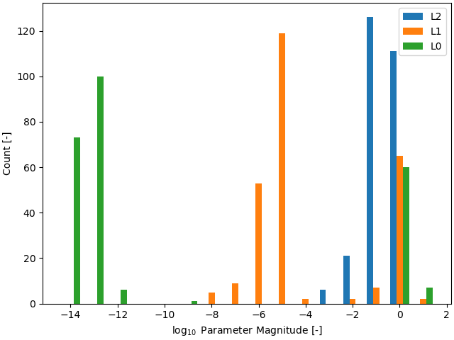
We can quantify this by plotting a histogram of the magnitudes of the transient parameters for the three different regularization schemes. One last time, we save the parameter values:
>>> params_transient_L0 = stat.models["Displacement"]["Transient"].parameters.ravel().copy()
>>> ZERO = 1e-4
>>> print("Number of nonzero spline parameters:\n"
...       f"L2: {(np.abs(params_transient_L2) > ZERO).sum()}\n"
...       f"L1: {(np.abs(params_transient_L1) > ZERO).sum()}\n"
...       f"L0: {(np.abs(params_transient_L0) > ZERO).sum()}")
Number of nonzero spline parameters:
L2: 264
L1: 76
L0: 67
As we can see, the L0-regularized solver gives a more sparse solution than both the L1- and L2-regularized solvers. A histogram can show this to use more visually:
>>> plt.figure()
>>> bins = np.linspace(-14.5, 1.5, 17)
>>> stacked_params = \
>>>     np.stack([params_transient_L2, params_transient_L1, params_transient_L0], axis=1)
>>> plt.hist(np.log10(np.abs(stacked_params)), bins=bins, label=["L2", "L1", "L0"])
>>> plt.xlabel(r"$\log_{10}$ Parameter Magnitude [-]")
>>> plt.ylabel("Count [-]")
>>> plt.legend()
>>> plt.savefig(f"{outdir}/tutorial_2j.png")
Comparing specific parameters
Before we finish up, let’s just print some differences between the ground truth and our L0-fitted model:
>>> reldiff_sec = (mdl_coll_synth["Secular"].parameters
...                / stat.models["Displacement"]["Secular"].parameters).ravel() - 1
>>> reldiff_ann_amp = (mdl_coll_synth["Annual"].amplitude
...                    / stat.models["Displacement"]["Annual"].amplitude)[0] - 1
>>> reldiff_sem_amp = (mdl_coll_synth["Semi-Annual"].amplitude
...                    / stat.models["Displacement"]["Semi-Annual"].amplitude)[0] - 1
>>> absdiff_ann_ph = np.rad2deg(mdl_coll_synth["Annual"].phase
...                             - stat.models["Displacement"]["Annual"].phase)[0]
>>> if absdiff_ann_ph > 180:
...     absdiff_ann_ph -= 360
>>> absdiff_sem_ph = np.rad2deg(mdl_coll_synth["Semi-Annual"].phase
...                             - stat.models["Displacement"]["Semi-Annual"].phase)[0]
>>> if absdiff_sem_ph > 180:
...     absdiff_sem_ph -= 360
>>> print(f"Percent Error Constant:              {reldiff_sec[0]: .3%}\n"
...       f"Percent Error Linear:                {reldiff_sec[1]: .3%}\n"
...       f"Percent Error Annual Amplitude:      {reldiff_ann_amp: .3%}\n"
...       f"Percent Error Semi-Annual Amplitude: {reldiff_sem_amp: .3%}\n"
...       f"Absolute Error Annual Phase:         {absdiff_ann_ph: .3f}°\n"
...       f"Absolute Error Semi-Annual Phase:    {absdiff_sem_ph: .3f}°")
Percent Error Constant:               7.264%
Percent Error Linear:                -1.378%
Percent Error Annual Amplitude:       2.308%
Percent Error Semi-Annual Amplitude: -0.407%
Absolute Error Annual Phase:         -1.836°
Absolute Error Semi-Annual Phase:    -1.284°
As we can see, we got pretty close to our ground truth. Let’s finish up by calculating
an average velocity of the station using get_trend() around
the time when it’s rapidly moving (around the middle of 2002). We don’t want a normal trend
through the data, since that is also influenced by the secular velocity, the noise, etc.,
so we choose to only fit our transient model:
>>> trend, _ = stat.get_trend("Displacement", fit_list=["Transient"],
...                           t_start="2002-06-01", t_end="2002-08-01")
>>> print(f"Transient Velocity: {trend[0]:f} {ts.data_unit}/D")
Transient Velocity: 0.105952 mm/D
We can use average velocities like these when we want to create velocity maps for certain episodes.